Mine is better: Metrics for evaluating your (and others) Machine Learning models

In our daily life, we all tend to use Accuracy and Precision as synonyms. In this great blog you can find a brief and clear explanation of the differences between them. Though this confusion does not pose a real problem in most day-to-day activities, when evaluating a Machine learning model, we cannot be that loose. We need to clearly understand what our metric is telling us about our model and be aware of the advantages and disadvantages of the metrics used. Though many people commonly brag about models with 98% or even 99% accuracy/precision, this statement can be very misleading. For example, let’s suppose we want to predict the Runway Excursion of an aircraft landing at our airport. Only 1% of all landings at our airport suffer a runway excursion. If we end up creating a model that predicts that all landings will not suffer a runway excursion, we would still end up with a model that has an Accuracy of 99%. Impressive right? For someone who is only given this metric without any more context, the problem may be difficult to detect. For that reason, this post specifically focuses on a brief and clear description of the main metrics you can use to evaluate your Machine learning model: Classification or Regression.

Classification Models:

Classifiers are a type of supervised learning model in which the objective is simply to predict the class of given data value. There is a great variety of classification models such as Logistic regression, K-Nearest Neighbors (K-NN), Support Vector Machine SVM or Decision trees. To try and help us understand the different evaluation metrics, I am going to propose a use case scenario as an example. In our case,the scenario we would be an airline that wants to predict if a passenger is going report to flight (1) or if he is going to no-show (0).

1. Confusion Matrix:

A Confusion matrix is simply a table that describes the performance of a classification model (outputs can be of two or more classes). This matrix is generally very intuitive and relatively easy to understand although some of the concepts and terminology surrounding it can be tricky at times. (Maybe that’s why it has “Confusion” in its name?)

Interpreting the Confusion matrix:

True Positive (TP): When our model predicts a “1” and the actual data is also a “1” → A passenger that is predicted to report to a flight and does so.
True Negatives (TN): When our model predicts a “0” and the actual data is also a “0” → A passenger that does not show up for a flight and was predicted to no-show.
False Positive (FP): When our model predicts a “1” and the actual data is also a “0” → A passenger is predicted to report for a flight but is actually a no-show. Also known as Type I Errors.
False Negative (FN): When our model predicts a “0” and the actual data is also a “1” → A passenger is predicted to no-show but actually reports to the flight. Also known as Type II Errors.

A perfect model would be that which has 0 False Positives and 0 False Negatives, but this is practically impossible in reality. When assessing the results, there is no standard action plan to follow on what you should minimise. This would depend completely on the business scenario you are working on. In the case scenario proposed, we can imagine that it is more costly for an airline to have a passenger overbooked (compensations, bad press, etc.) than a seat being empty on the flight. Therefore the airline should focus on reducing False Negatives more than the False Positives.

Below you will find an awesome visualization made by Data Plus Science in Tableau that you can interactively explore to better understand a Confusion Matrix. You can change the cut-off value of the classification varying the False Positive and False Negative rates. You would also see how this variations change the Precision and Accuracy.

2. Accuracy:

Accuracy is simply the correct number of predictions made over all the predictions made by the model.

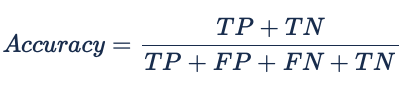
As mentioned before, accuracy is a metric that must be used with a lot of caution as it can be misleading if used solely. This metric is most useful when we are working with balanced datasets.

3. Recall vs Precision:

Recall (or Sensitivity): This metric tells us how well our model predicts the positive (1) events of our data. In our case scenario, it would show us the proportion of passengers that report to the flight and that were predicted correctly by the model.

Precision: How often is our model correct when it predicts a positive (1) event. When we predict that a passenger is going to report to the flight, how often does it get it right.

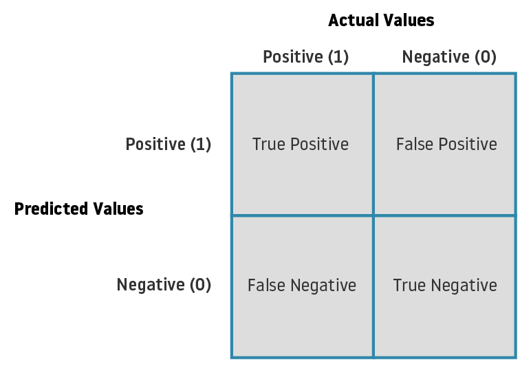
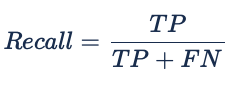
Precision can be seen as a metric that gives us information of how well our model performs with regard to the False Positives. Recall, similar to precision, gives information about the performance with regards the False Negatives. In our case scenario, we are more interested in minimising False Negatives (passengers overbooked) so we are looking for as big of a Recall as possible without overlooking Precision. If our model predicts all passengers as positive (1) events, our Recall would be 100%. But what could occurs is that our flights, due to no-shows, have a load factor inferior to the Break-even load factor which is bad for the revenue.

4. Specificity:

Specificity is the complete opposite of Recall. This metric tells us how well is our model in predicting the negative (0) events of our data. In our case scenario, it would show us the proportion of passengers that do not finally show up that were predicted correctly by the model.

5. F1 score:

F1 score is a metric that combines both Precision and Recall. This combination is made using the Harmonic mean.

The use of the Harmonic mean, in contrast to the arithmetic mean, makes the F1 score metric more sensible to the differences between Recall and Precision, making it lean closer to the smaller of both numbers. Some of the main concerns raised in using this metric are that it gives the same relevance to Precision and Recall (False Positives and False Negatives). In reality, as mentioned before, there can be different costs for the possible misclassifications (overbooking vs Empty seats).

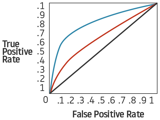
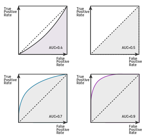
6. AUC-ROC Curve:

AUC (Area Under Curve) is almost certainly the most used metric for the evaluation of binary classification models. ROC ( Receiver Operating characteristic Curve) is the most common way of visualizing how well a classifier works.

ROC: Is basically a graph where True Positives and False Positive values are plotted for all possible classification thresholds [0…1]. An example of a ROC to classifiers (Blue and Red) can be seen in the image below. In this link, you can find a wonderful visualization of an ROC which you can interact with to better understand how it is constructed.

AUC: As the name suggests, this metric is nothing more than the value of the area that is under the ROC of your model.

The range of values you can obtain with AUC are from 0 to 1. The bigger the value of AUC, the better your classifier. If the model that we created for our case scenario predicted all passengers wrongly, then its AUC would be 0. By contrast, if our classified correctly predicted all passengers, then it would have an AUC of 1. One of the main strengths of the use of AUC is that it is independent of the scale of the measures of the classifier. Another of the strengths of the AUC metric is that it is independent of the threshold of the classifier, although this could introduce a problem if there is a big cost contrast between False Positives and False Negatives.

Regression Models:

Regressions are a type of supervised learning model in which what we want to predict is continuously valued. Some of the regression algorithms that exist are Ridge Regression, Regression trees or Support Vector Regression (SVR). As with the Classification models, to try and help us understand the different evaluation metrics, I present an example – we are going to be an Airport Operator and we would like predict the ROT (Runway Occupancy Time) of the aircrafts landing at our airport.

1. MAE:

MAE (Mean absolute Error) is one of the most basic and easy-to-understand error metrics for regression models.

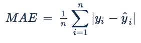
MAE is simply the average of the difference (as an absolute) between the predicted values and the actual data (see the formula below). The main characteristics of this metric are that as it uses the absolute and does not take in account the direction of the error (the metric does not depend on the real ROT being faster or slower than the predicted) and that all individual errors are weighted equally in the average (all errors have the same importance).

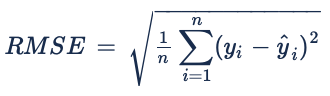
2. RMSE:

RMSE (Root Mean Square Error) is, in some way, similar to the MAE as it is also mainly based in the difference between the prediction and the actual data.

There is a lot of debate whether to use MAE or RMSE when evaluating a model. Both metrics are indifferent to the direction of errors and the lower the values of the error, the better the model. The main difference between both metrics is how they respond to large error. Let’s use an example of the case study proposed. We have 5 aircrafts that have landed in our airport with the next ROT [40, 51, 57, 43, 61] and our models give these corresponding predictions [45, 48, 64, 47, 57]. The errors for our model would be: MAE = 4.8 and RSME = 5.1. Choosing one over the other comes again to a business decision and the cost associated to the errors. If the cost of the error does not increase considerably with the value of the error then MAE could be more appropriate, but if the cost associated with a large error is big, then it maybe better to use RMSE to evaluate your model. In our case study, predicting an ROT that is considerably higher than the real one would have the cost of underusing the runway capacity. On the other hand, a considerable lower ROT prediction could cause a safety incident, which is a really high cost for the airport. So in our model it seems wise to more severely penalize the big errors. In that case, RMSE would be more appropriate to use.

I hope this blog has helped you better understand the main metrics available to evaluate Machine Learning models as well as raised awareness of the advantages and disadvantages of each. In the end, each metric provides you with a specific picture of the performance of your model. You are the one that has to decide which metric (or metrics) best helps you ensure your model is working the way you desire. At least now you will be skeptical the next time someone presents a model with 99% Accuracy. Do not forget to visit other fantastic blogs in datascience.aero to learn and discover new things about the wonderful world of Data Science and Aviation.

Mine is better: Metrics for evaluating your (and others) Machine Learning models

Pablo Hernández