Hyper-parameters, learning rates or activation functions are good examples of concepts that sound familiar in almost any Deep Learning scenario. When Data Scientists design an Artificial Neural Network (ANN) layers architecture, new concepts and customizable parameters will appear, providing a lot of flexibility to adapting general neural network archetypes to a particular use case. Nevertheless, sometimes the extensive amount of configurable values complicates the network optimization task, requiring advanced knowledge and experience in training neural networks. This sometimes prevents engineers from extracting the full potential of deep learning. In this post, we are going to explain the activation functions concept in depth and analyze which case studies might benefit from using them.

Activation functions represent a key factor in ANN implementation. Their main objective is to convert an input signal of a node to an output signal and are known as transformation functions for this reason. If we don’t apply an activation function to network layers, the output would be transformed into a linear function, leading to many limitations due to their low complexity and capacity to learn complex and intrinsic relationships among dataset features. Non-linearity is predominant in real life datasets. For example, images, voice recordings or videos can’t be modeled following this simple approach as they are composed of multiple dimensions that can’t be represented with linear transformations. Differentiability is another property of activation functions, which is mandatory to perform back-propagation optimization strategy. In the context of learning, back-propagation is normally used by the gradient descent optimization algorithm, which adjusts the weight of neurons by calculating the gradient of the loss function. For back-propagation, the loss function calculates the difference between the network output and its expected output after a training observation has propagated through the neural network.

Almost all activation functions struggle with a very well-known issue: the vanishing gradient problem. As more layers using a certain activation function are added to a neural network, the gradients of the loss function begins to approach to zero, freezing the network training. This, in turn, becomes a very hard issue to solve. Since back-propagation finds the derivatives of the network by moving layer-by-layer from the last layer to the initial one, according to the chain rule statements, the derivatives of each layer are multiplied down the network. A small gradient (near zero) implies that the weights and biases from the first layers won’t be updated effectively while training the network, and this can lead to a loss of accuracy since the model is unable to recognize core elements from the input data, which often occurs at network entrance.

With these premises, you might be asking the following questions: in which situations is it preferable to use one activation function over another? Is any non-linear function allowed to activate neurons? What requirements should be achieved by activation functions to avoid the vanishing gradient problem and to allow deep learning techniques to be able to solve a predictive case?

In which scenarios should we use one activation function instead of another?

For simple scenarios, use conventional functions

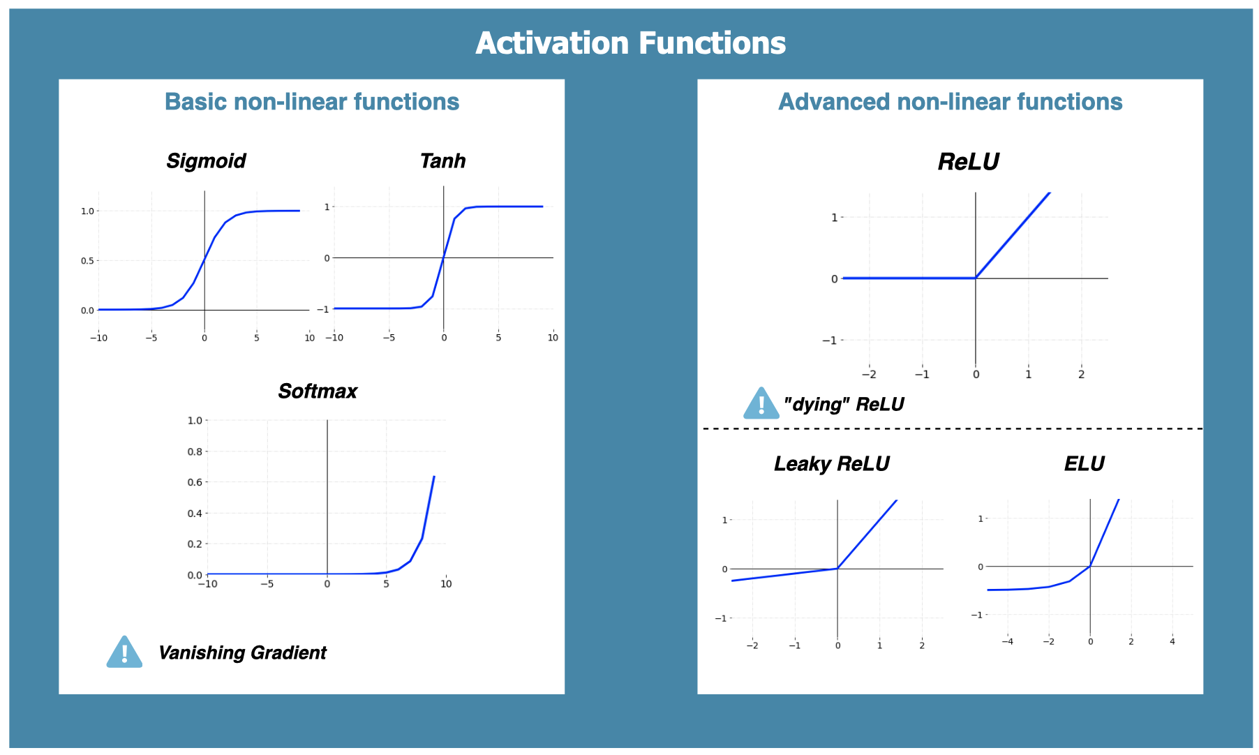
Sigmoid is an activation function whose range is located between 0 and 1, and it generally works better when we have to predict the probability as an output in logistic regression scenarios to determine the probability of classes occurrence. Also notice that the sigmoid function is centered between 0 and 1, making the gradient updates go too far in different directions, which in turn makes optimization a bit harder than using other activation functions. The decision threshold can be directly extracted from the graphical representation of the function, if X→−∞X→−∞, it can be classified as 00, and, on the other hand, if X→∞X→∞, the output will be 11. The main problem when using sigmoid as activation function is that they are affected by the vanishing gradient problem, and therefore must be used only for networks composed of a low number of layers. 

Tanh function graphically looks very similar to sigmoid apart from being centered between -1 and 1. The main advantage of this is that the negative inputs will be mapped strongly negative and the zero inputs will be mapped near zero. The tanh function is mainly used in scenarios where we want to perform a classification between two classes. Regrettably, this activation function is also affected by the vanishing gradient problem, so network layer size must be considered.

Softmax is a more generalized logistic activation function mostly used for classification problems in which we have multiple classes, not just binary. It is able to map each output in such a way that the total sum is equal to 1. Since the output is a probability distribution, softmax is normally used in the final layer of a neural network classifier.

To summarize, conventional activation functions are mostly used in the following scenarios:

• softmax is used for multi-classification in logistic regression models
• sigmoid and tanh are used for binary classification in logistic regression models

For linear regression case studies, activation functions are not needed in output layers as we are mainly interested in specific numerical values (continuous) without any transformation.

For more complex scenarios, better use ReLU

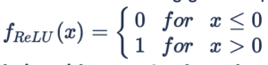
ReLU (Rectified Linear units) is a very simple and efficient activation function that has became very popular recently, especially in CNNs. It avoids and rectifies the vanishing gradient problem, which mostly explains why it’s used in almost all deep learning problems nowadays. The gradient for ReLU is:

Hence multiplying several ReLU derivatives together in the back-propagation equations which have the nice property of being either 1 or 0, where the update is either nothing, or takes contributions entirely from the other weights and biases. This allows a network to easily obtain sparse representations with a relatively small number of useful links, since, as ReLU is zero for all negative inputs, it’s likely for any given unit to not activate at all.

But why is sparsity good for the model? ANNs behave analogously to biological neural networks, where neurons have different roles and are activated by different stimuli. Having sparsity in ANNs leads to a more concise model, less overfitting and better accuracy in prediction output. Within a sparse network, neurons actually process meaningful information regarding the problem to solve. A clear example would be face recognition, where a neuron might be responsible for identifying eyes, which shouldn’t be activated if the image is about vehicles.

ReLU is cheap to compute and takes less time to train or run as a model, having fast convergence and being sparsely activated. However, the downside for being zero for all negative values is a problem called “dying ReLU.”

The “dying ReLU” problem

The main inconvenience for ReLU is the “dying ReLU” problem caused by return zero for all negative inputs. A ReLU neuron is “dead” if it’s stuck in the negative side and always outputs 0. Since the slope of ReLU for negative range is always 0, once a neuron enters that area it’s unlikely for it to recover, basically being useless for learning. This problem usually occurs when the learning rate is too high or if there is a large negative bias.

Emerging ReLU variants to solve this problem

Leaky ReLU and PReLU (Parametric ReLU) introduce few modifications to ReLU. Both alternatives provide a small slope for negative ranges, static for Leaky ReLU, and as a parameter for PReLU. This way, the “dying” ReLU problem is completely solved as it doesn’t have zero-slope parts. They also slightly speed up training, being more balanced and learning faster. These alternatives might be considered for scenarios where the training process takes too long, in order to avoid inactive neurons in the network.

Similar to leaky ReLU and PReLU, both ELU and SELU provide a small slope to negative values, but using an exponential curve. They mix elements of basic ReLU and Leaky ReLU, since they provide negative values in the short-term, but remain inactive for large negative values in the long-term.

Conclusion: ReLU will probably fit with your problem

To sum, ReLU offers the best solutions over other alternatives and is normally used as a first-approach to almost any deep learning problem. While optimizing the neural network, it’s a good practice to at least prove any other ReLU variants and evaluate the improvements in accuracy, training time and resources consumption. As new functions are constantly appearing, it’s important to identify which better adapts to your problem, and, moreover, to evaluate multiple combinations while designing your network layers and tuning hyper-parameters.

Read more deep learning posts in datascience.aero

Aviation revolution nears with Artificial Intelligence and Deep Learning